The Genome-wide Signal of Linked Selection in Temporal Data
The last chapter of my dissertation with Graham Coop was recently published in PNAS (pdf, bioRxiv) last week. In an effort to communicate my research to a broader audience, I have written two blog posts on our work. The first post, is meant to introduce the historical context and concepts like linked selection and polygenic adaptation to a non-scientist, and the second post, below, describes our work on temporal covariance as a signature of polygenic linked selection and its application to four evolve-and-reseqeunce data sets.
In the last post, I explained two longstanding problems in the field of evolutionary genetics. The first is detecting adaptation on polygenic traits from temporal genomic data. Temporal data is gathered by sampling a population through the generations and sequencing these samples, and provides us with a immense amount of information about the evolutionary process over short timescales. Yet even with this amount of data, distinguishing allele frequency changes caused by polygenic selection from that random genetic drift is a challenge. A population could be adapting over short timescales —we might even observe drastic changes in a trait over a few generations— yet it could be impossible to see the signature of such strong selection at the DNA level.
The second related problem is how we quantify the roles of drift and linked selection in determining genome-wide allele frequency changes. Since the debates between Fisher and Ford, and Wright, evolutionary geneticists have disagreed on the relative roles played by genetic drift and natural selection in determining allele frequency changes. Since their time, we have learned selection at a site exerts a strong influence on its linked neighbors, known as linked selection. This perturbs the frequency trajectories of alleles through time, and to have a complete view of how populations evolve we need to understand this process. With temporal data, we could perhaps directly estimate the effects of linked selection on drift on allele frequency change.
The Quantitative Genetics View of Linked Selection and Temporal Covariance
In our first paper (Buffalo and Coop, 2019), Graham and I proposed that one promising signal that could be used to detect polygenic selection in temporal genomic data is temporal covariance. Our work builds of many excellent papers but three in particular: Robertson (1961), and Santiago and Cabarello (1995, 1998)1.
These papers (and others) establish what I’ll refer to as a quantitative genetics view of linked selection, and implicitly describe temporal covariance. While the classic linked selection work (i.e. hitchhiking and background selection, which I explain in the first post) describes how a neutral allele behaves when it is a close neighbor of a new mutation that affects fitness, the quantitative genetics view of linked selection often seeks to understand how a neutral allele behaves when it is much more distant —perhaps even on a different chromosome— from the genetic variation that is selected upon. Furthermore, this view supposes the genetic variation that determines fitness is polygenic, and results from standing variation, meaning it is present at appreciable frequencies in the population (i.e. not the rare new mutations of the classic linked selection work).
Figure 2 Wright’s (1940) figure of extinction and recolonization in a population. Population lineages are expanding through time from left to right and space (top to bottom), with groups going extinct and re-establishing. The genetic drift in a population with such a complex breeding process can be represented by standard population genetic models with a rescaled effective population size.
One of Sewall Wright’s ingenious ideas was to recognize that many different breeding structures we might see in nature (e.g. organisms capable of self-fertilization, or the extinction-recolonization dynamics depicted above) can still be described by standard models of genetic drift, as long as the population size is rescaled appropriately. We call this effective population size2, and the early work of Robertson first described the long-run effect of selection on a polygenic trait exerts on a neutral site as a reduction in effective population size. This, in essence, means selection can make it seem genetic drift is running faster since changes are larger per unit time. The fact that many types of selection have effects quite similar to random genetic drift occurring in a smaller population is one reason why the effects of selection and drift can be hard to distinguish. This is precisely why Fisher and Ford first had to estimate the population size to test whether selection caused the decline in frequency of the dark wing color variant: they needed to determine the magnitude of genetic drift to see if the frequency changes were too drastic to be caused by drift alone, and were more likely to be caused by selection.
While Robertson, and Santiago and Cabarello’s work expressed the linked selection effects felt by a neutral allele during polygenic selection as a reduction in effective population size, their work tells us there is one key difference between a neutral allele randomly drifting in the population, and a neutral allele affected by linked selection: with linked selection, the neutral allele’s frequency changes between two generations are correlated with the changes between later generations. Imagine following a neutral allele as it descends down lineages, forward through the generations towards the present. In one generation, the neutral allele finds itself in a father carrying genes very well suited for his environment, and as a result, he leaves many offspring. Each child inherits some fraction of his well-suited genes, and possibly, the neutral allele as well. Within this family, the neutral allele’s frequency increases. As long as the genes that suited him well in this environment are also beneficial in his children’s generation, they too will leave more offspring. So too will the neutral allele’s frequency also rise in this generation, as long as it remains associated with a fraction of genes well-suited for this environment.
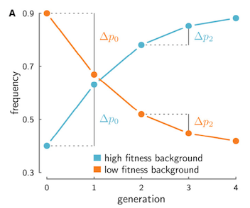
If we were to track this neutral allele’s frequency trajectory through time in the entire population, we would see it rise between the two first consecutive generations, and then rise again between the next two, as long as it remains associated with a fraction of the father’s beneficial genes. The neutral allele’s frequencies between the second and first generation (mathematically, \(\Delta p_1 = p_2 - p_1\)), and the third and second generation (\(\Delta p_2 = p_3 - p_2\)) would both change in the same direction when they’re associated with this good background, creating temporal covariance in the frequency trajectory. This same effect happens if the neutral allele were to instead be associated with a disadvantageous background (see figure above). In contrast, genetic drift cannot create temporal covariance in neutral allele frequency trajectories. Another way to say this is that when different chromosomes have heritable fitness differences, the frequency change of an allele at one time interval can be predictive of the changes at later generations, as long as the allele is still associated with its fitness background, and that background has the same effect on fitness.
In Buffalo and Coop (2019), we proposed using temporal genomic data to quantify the amount of temporal covariance in a population, and use it as a means of detecting polygenic selection over short timescales. We also develop a mathematical theory of what determines the strength of temporal covariance, and find it is determined by how much additive genetic variance for fitness there is in a population (a key quantitative genetics parameter), and how strong the neutral allele’s association is with the genetic fitness variation (which is mediated by the level of recombination and the strength of initial association, known as linkage disequilibrium).
Detecting Temporal Covariance in Evolve-and-Resequence Studies
With a basic understanding of how temporal covariance functions as a signal of polygenic selection, let’s look our recent paper, Buffalo and Coop (2020). In this study, we applied the methods we developed in our Genetics paper to four evolve-and-resequence studies. Our work relied entirely on the accessibility of the data from these previous studies, and we both are grateful for the authors’ support and openness with their data.
The first study we analyzed was from Barghi et al. (2019), an evolve-and-resequence study in Drosophila simulans. In this experiment fruit flies were evolved in a hot laboratory environment for 60 generations, across ten independent replicates. We re-analyzed this well-designed study using our temporal covariance methods. We found extensive evidence of temporal covariance through time (Figure A below), consistent with the original author’s findings that the populations were adapting to their new warmer environment. Furthermore, these temporal covariances declined through time, just as we expected, since the temporal covariances weaken as the associations between neutral sites and fitness variation decay through time.
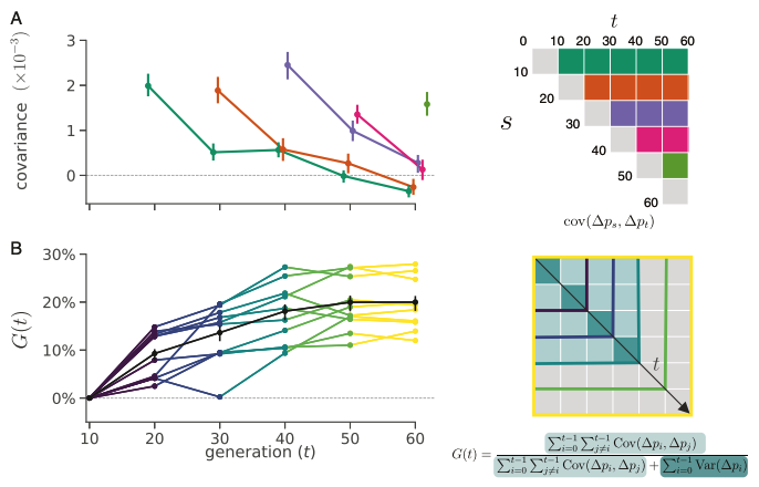
In Buffalo and Coop (2019), we proposed that we could use temporal covariances to estimate what proportion of total variation in allele frequency change is caused by linked selection2. We called this proportion \(G\); if \(G = 0\), all the variance in allele frequency change is caused by genetic drift, whereas if \(G = 1\), all the allele frequency change is caused by linked selection. We calculated \(G\) as it accumulates through the generations (and thus call it \(G(t)\) where \(t\) represents time), shown in the Figure B above. Because samples in Barghi et al. (2019) were sequenced every ten generations, our \(G\) estimate is a lower bound estimate, meaning the actual proportion of variation in allele frequency change due to linked selection is higher than our \(G\) estimates. Still, we find that over short timescales, at least 20% of the variation in allele frequency change is due to linked selection. This provides us with the first glimpse of how linked selection determines frequency changes over very short timescales.
Given we find such evidence of linked selection over short timescales, two questions arise: (1) is this really polygenic selection? and (2) where is the signal coming from? First, to investigate whether this was indeed polygenic selection, rather than selection on a few mutations that have large effect, we calculated temporal covariances along windows in the genome. If our genome-wide signal of linked selection was driven by a few regions under strong selection, we should expect to see these regions as outliers. Instead, we see that the whole distribution of windowed covariances is enriched for positive covariances, indicating the signal we’ve detected is spread across the entire genome.
Second, how can we detect a signal of linked polygenic selection when the effect at each site is so weak? Drift and sampling variance introduce considerable noise that can swamp the signal of temporal covariance, as well as create spurious covariances. However, these sources of noise do not share random change in the same direction, whereas temporal covariances do, leading to a signal that can be readily distinguished from random drift.
Convergent Correlations
One common study design of evolve-and-resequence experiments is to evolve multiple indepedent populations under the same (or different) environments, and look for evidence of convergent (or divergent) selection. We hypothesized that we should be able to detect something analogous to temporal covariance across replicate populations exposed to the same selective pressures. This is because replicate populations created from the same founding population will, by chance, share some of the same fitness variation. Neutral alleles associated with the same advantageous genetic backgrounds would then be expected to increase in frequency through time, in both replicate populations. This creates what we call between-replicate covariance, and we can measure this much like we do temporal covariance.
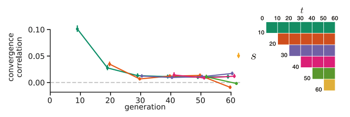
The Barghi et al. study evolves ten replicate populations independently, which provided us with a great data set to see if we could detect between-replicate covariances. To measure the extent of between-replicate covariances, we use what we call convergence correlations, which are simply the covariance in allele frequency changes between replicates scaled by the standard deviation in allele frequency change. As with our temporal covariances, we calculate these for all time intervals, and find that they are relatively week and decay quickly through the generations. This tells us that while early on, the selection occurring across replicates is similar, each replicate quickly goes its own way (and this confirms a major finding of the original Barghi et al. study, that different loci across replicates contribute to adaptation).
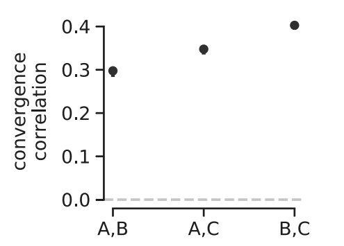
A benefit of convergence correlations is that unlike temporal covariances, they only require evolve-and-resequence studies with two timepoints and replicate populations. This allowed us to re-analyze two other elegant evolve-and-resequence studies. The first is Kelly and Hughes (2019), which evolved three replicate populations of Drosophila simulans to a novel lab environment. Similar to our re-analysis of the Barghi et al. study, we calculated convergent correlations across each pairwise combination of the replicate populations and find that all these convergent correlations are statistically significant and stronger than those we see in the Barghi et al. study3. Furthermore, using an approach like \(G\) described above, we found that at least 37% of the total variation in allele frequency change was shared between replicates, which is a pretty sizable proportion considering these lab populations are rather small and strongly affected by genetic drift.
The second study is Longshanks selection experiment of Castro et al. (2019, see also Marchini et al. 2014), where over twenty generations, two independent replicate population lines of mice were selected for longer tibiae lengths relative to body size. The study also has a control line, where mice were bred randomly. Remarkably, over twenty generations of selection, tibiae length increased about five standard deviations.
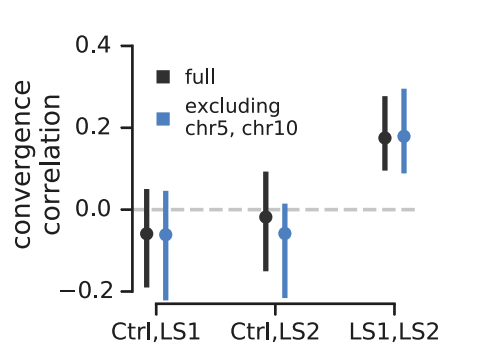
Since the Longshanks study has a control line, it provided a powerful test of our convergence correlations: we should expect significant convergence correlations between the two Longshanks selection lines, but not between each Longshanks selection line and the control line, since these two do not share convergence selection pressure. This is precisely what we find (shown above). Furthermore, the original Castro et al. study found two large effect loci, one on chromosome 5 and the other on chromosome 10. In the original paper, they show that while the loci on these chromosomes show a signal of convergent selection, the trait itself is highly polygenic. In sharing our preliminary results with the authors of Castro et al., they wondered the extent to which our convergence correlations were driven just be these large-effect loci. We decided to exclude these large-effect loci by leaving out the entire chromosomes they reside on (in part, because these loci could have far-reaching effects on linked variation). We show the convergence correlations sans these chromosomes above in blue — they are also statistically significant, indicating the signal we are detecting is polygenic.
The presence of the control line also allowed us to do a fun little calculation to partition the total variation in allele frequency changes into drift, shared selection, and unique selection components. Since the mating of mice is random in the control line, the total variance in allele frequency change we see is due only to genetic drift. Any additional variance in allele frequency change we see in the two control lines is then caused by selection (due to exactly the same effect that Robertson 1961 described). Furthermore, we can estimate the fraction of variance shared between the Longshanks selection lines, since this is just the covariance in frequency changes between Longshanks lines. Finally, the remaining part of the variance due to selection is that which is unique to each selection line. We find that at least 32% of the variance in allele frequency change is due to selection, and of this 32%, 17% is due to shared selection pressures and the remaining 14% is due to unique selection pressures or associations unique to a particular replicate population3.
Shifts in Temporal Covariance
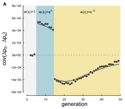
In our Genetics paper, we suggested that fluctuating selection could create negative temporal covariance. The intuition here is that if a neutral allele rises in frequency on a beneficial genetic background, a change in the environment that leads this background to become disadvantageous would cause a decline in frequency. Since in the first generations \(\Delta p_t > 0\) and in the later generations \(\Delta p_s < 0\), the temporal covariance would be negative (see figure above). We confirmed this hunch with simulations in our Genetics paper, and were curious if we’d see this pattern in real data.
If you look closely at Figure 4 (A) above, you’ll see that at later timepoints, we do observe negative covariances that are statistically significantly different from zero. This is consistent with a reversal in the fitness of certain genetic backgrounds. We wondered to what extent these reversals at later time intervals were common, but obscured since we were average over the entire genome.
One thought we had was that perhaps we could look for such reversals happening in smaller chunks, or windows, of the genome. While this could allow us to detect subtle, local reversals in selection dynamics, it introduces two problems. First, the temporal covariance estimates are incredibly noisy, since we’re averaging over fewer sites. Second, we would need a way to estimate what the distribution of these temporal covariances across windows would look like under just drift, as a null hypothesis. We devised a simple way to do this by randomly permuting the allele frequency changes across each window, and looking at the entire distribution of windowed temporal covariances. The permutation approach essentially breaks the directionality of temporal covariances caused by selection, and gives us an estimate of the distribution of temporal covariances as they would be under just genetic drift, which we could compare to our observed distribution. Below, I show the distributions of the windowed temporal covariances between different time intervals:
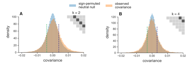
In Figure 9 (A) above, the temporal covariances are separated by two timepoints (20 generations), and we see an enrichment of positive temporal covariances across the genome, consistent with the findings mentioned above. In Figure 9 (B) above, the temporal covariances are 40 generations apart and we see an enrichment of negative covariances, compared to the null distribution in blue. Our paper and the appendix shows more figures illustrating this point. Seeing the signal of such selection dynamics over short timescales was an unexpected and interesting surprise. Note that the environment in the Barghi et al. study was kept constant; there was not an any outside factor that was intentionally changed that could lead to such a reversal in the direction of selection. This tells us that rather complex selection dynamics could be common over short evolution, and these selection dynamics may go unnoticed in the long-run despite having a considerable impact on genome-wide frequency changes.
Conclusions
Overall, we find that as sizable proportion of allele frequency change, over short timescales, is due to selection (likely through its effects on linked sites). Our approach was overall extremely conservative, so the actual effect could be much greater. As further evolve-and-resequence studies are designed and conducted, I hope to apply and improve these methods to get better estimates of the impact of polygenic selection on genome-wide frequency changes. Overall, I believe our view of evolutionary genetics will be greatly advanced if we continue to try to understand genomic evolution over short timescales and try to reconcile these with population genomic studies using samples from a single contemporary timepoint.
Our paper contains much more detail, and many analyses I’ve omitted here for brevity. I have left out our entire section on the extensive simulations we have conducted using SLiM, which confirm that our measures of temporal covariance, \(G\), and convergence correlations work as intended. Graham and I are both quite grateful to our reviewers and our editor for a recommendations and a review process that made our paper much stronger.
Finally, I should point out that this entire project was only possible because the authors of the original studies conducted careful, well-designed experiments, and were open with their data. I am extremely grateful for this openness and I hope our re-analyses bring their excellent papers more readers. Following their lead, I have made my analyses and the intermediate data I produced openly available on Github. Each analysis was conducted in a Jupyter Lab notebook using open source tools, and I have tried to make my analyses as reproducible as possible. Collectively, our knowledge of evolution will grow faster if we all embrace the same open science mindset.