Why Do Species Get a Thin Slice of π? Revisiting Lewontin’s Paradox of Variation
The Great Obsession of population geneticists, to borrow John Gillespie’s words, is genetic variation. As an evolutionary biologist, it’s rather hard to not be obsessed with genetic variation, for it’s the ultimate source of the two most striking features of life on earth: the mind-boggling diversity of species, and adaptations so utterly clever they look as though they were assembled by a designer. Both life’s dizzying diversity and cunning adaptations are the result of evolutionary processes like natural selection and numerous historical accidents, overlaid on one another like brush strokes on canvas, to give us the snapshot of life on earth today.
Population geneticists’ obsession with genetic variation is a result of the way we look at evolution: evolution as the change in the genetic composition of a population through time. By carefully studying genetic variability, we hope we have some chance of figuring out which evolutionary processes played out in the past. Some biologists dismiss this view as “beanbag genetics”, since population geneticists like to reduce a population down to the simplest components: the frequencies of various genetic variants, or alleles, in that population. While surely this is an oversimplified view, the upside is that it is particularly amenable to thinking about mathematically. Indeed evolution often occurs so slowly that to understand it we need to use mathematics to figure out what a population looked like long before we were born, or what it will look like long after we’re dead.
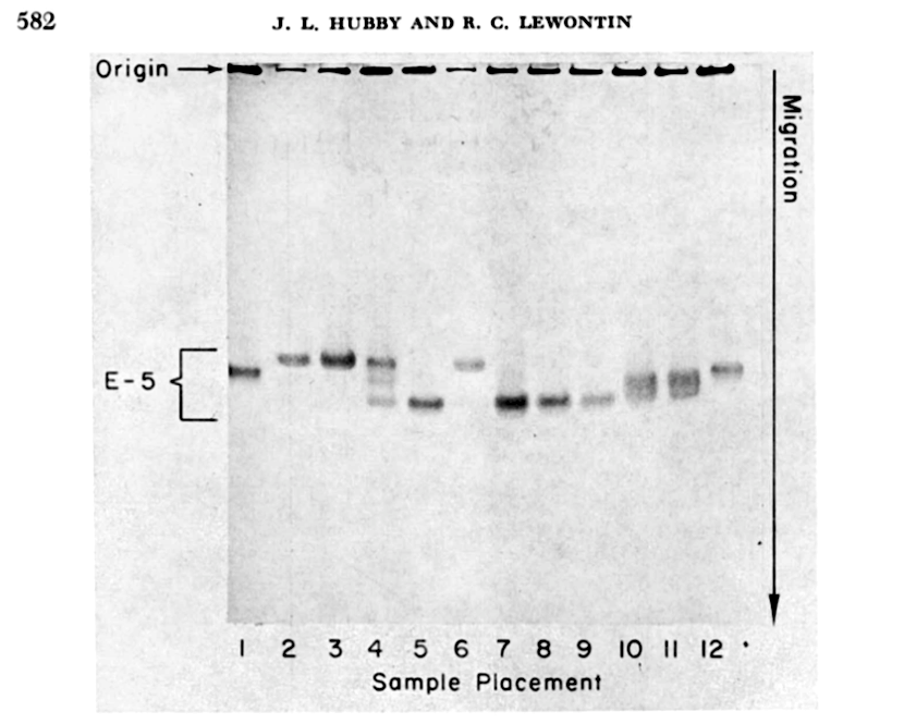
Our field has constructed a rich mathematical theory of evolution over the last one-hundred years, but it was only a half-century ago we got our first actual estimates of the genetic variation in a fruitfly species named Drosophila pseudoobscura, from the work of Richard Lewontin and Jack Hubby. After a glimpse of the data, one theory of evolution was slain, and its rival theory was in disarray. Within a few years, evolutionary biologists were measuring genetic variation in all kinds of species during the “find ’em and grind ’em” era, named for the unceremonious way numerous flies, crabs, plants, and individuals from other species met their fate in the quest to measure variability.

With new data of levels genetic variability across species, another theory was soon on chopping block. This theory was the neutral theory, and Dick Lewontin’s 1974 synthesis of the find ’em and grind ’em era pointed out a seeming contradiction between this theory and the new estimates of genetic variability. He named this the “The Paradox of Variation”, and it’s an enduring riddle in my field of evolutionary genetics. My recent paper published in eLife attempts to make some progress on this longstanding paradox. I’ve written this blog post to introduce a general audience to these topics and why we study them, and then give an overview of my paper (you may wish to skip ahead and start there).
Lewontin and Hubby’s Quest to Measure Genetic Variability
Before Lewontin and Hubby’s work measuring genetic variability in Drosophila pseudoobscura, evolutionary biologists were uncertain of how high or low the genetic variability was within populations. As I write this, I am surrounded by two examples of the extremes of this genetic variability spectrum: my Monstera deliciosa houseplant (also known as the Swiss cheese plant for it’s deeply fenestrated leaves) and the Drosophila fruit flies that have invaded the kitchen compost bin I’ve procrastinated emptying. While its incorrect to think of the monsetera plants in people’s homes as a “population” since they do not interbred with one another, they serve as a good example a group of organisms with low genetic diversity. This is because most monstera houseplants are clones of one another, created by taking a clipping of one plant, letting it root and grow, then taking a clipping of this plant, and so on. Unlike parent and offspring which are separated by a generation, all monstera plants are identical siblings; perhaps some mutations lead to small amounts of genetic variability, but this genetic variability is minuscule compared to what’s created by free mating in a sexually-reproducing species.
By contrast, my compost bin population of Drosophila melanogaster harbors massive amounts of genetic diversity. Part of the reason why Drosophila melanogaster have such high genetic variability is because their population sizes are so large. Drosophila melanogaster originated from equatorial Africa, yet followed humans around the globe living off our trash heaps and spoiled fruit. One way to measure genetic diversity is to take two random chromosomes and count the differences between their DNA sequences, then repeat this for another two random chromosomes, and so forth. Population geneticists call this “pairwise” measure of genetic variability the Greek letter \(\pi\) (I imagine much to the disappoint of mathematicians). For Drosophila, \(\pi_\text{flies} \approx 1\%\), or one difference per 100 DNA basepairs, and for humans, \(\pi_\text{humans} \approx 0.1\%\), or one difference per 1,000 basepairs. Humans have much lower genetic diversity than fruitflies. Lewontin and Hubby explain the drastic importance of this simple quantity:
In a sense, a description of the genetic variation in a population is the fundamental datum of evolutionary studies; and it is necessary to explain the origin and maintenance of this variation and to predict its evolutionary consequences. […]
Thus, one end goal of measuring variability within and across species is to answer the fundamental question of evolutionary genetics: what evolutionary processes are compatible with the observed levels of genetic variation?
The Evolutionary Theories Killed by Measuring Genetic Variation
Before I introduce Lewontin’s Paradox of Variation and the neutral theory, it’s worthwhile to set the stage with the theories of genetic variability that preceded it.1 At the time of Lewontin and Hubby’s work, proponents of the classical theory believed there wasn’t much genetic variation between individuals. This was because selection was thought to be extremely powerful: a new mutation that increased survival or the number of offspring quickly replaced all alternatives. The genetic composition of a population was more or less uniform, as it moves from one perfectly adapted state to another under the steady marching orders of natural selection. Of the variation that existed, it was primarily from harmful mutations that ‘broke’ organisms from their archetypal “wild-type”.2
By measuring their genetic variability, Lewontin and Hubby showed genetic variability was far too abundant for the classical theory to be correct. The alternative view, the balance theory, held that natural selection maintained vast amounts of genetic variation through a variety of mechanisms; aspects of this theory were successfully challenged through other experiments and arguments3. How evolutionary processes, whether random change, natural selection, historical accidents (e.g. a population bottleneck), combine to determine the central quantity of evolutionary genetics, genetic variation, remained a mystery.
The Neutral Theory
This brings us to the architect of the third view of genetic variation: Motoo Kimura. Kimura’s view was that the majority of genetic variation was selectively neutral: it did not impact the survival or number of offspring individuals had. Free from the marching orders of selection, such neutral variation lingered in populations, drifting up or down in frequency due the vagaries of which chromosomes were passed down to offspring (Mendelian segregation), and random differences in survival and offspring number that didn’t have a genetic cause. We call this process genetic drift. Kimura’s neutral theory was in some ways an extension of Sewall Wright’s view that evolution was governed as much, or more, by random chance as it was by natural selection. While here we’re focused on Kimura’s work on neutral polymorphism within a population, much of Kimura’s motivation for his neutral theory was to explain observations in molecular evolution, such as the steady clock-like ticking of amino acid differences between species.
Suddenly under neutral theory, the mystery of why there was so much genetic variation wasn’t such a mystery. If the variation was neutral, natural selection couldn’t act on it. Surely, some beneficial mutations would enter the population —adaptations of course had a genetic basis— but these mutations were rare, and they would quickly replace their alternative and didn’t persist for long in the population. Lewontin called neutral theory the “neoclassical theory” because of this similarity.
Setting Goddess Tyche in charge of evolutionary change has another benefit. If we can ignore natural selection, and thus all the uncertainty about the strength and direction of natural selection, the mathematics of evolution become much simpler. Under a model where \(N\) individuals freely mate, new variation is created through mutation at rate \(\mu\) per generation per basepair (i.e. there’s a \(100 \times \mu\)% chance that any one basepair mutates in a given generation), and new variation is lost through random drift at rate proportional to \(1/N\) (i.e. slower in larger populations, fast in small populations). Ultimately, like the level of water in a dam, a balance is met between new mutations entering and old mutations going extinct in the population: this is the equilibrium genetic diversity. A bit of mathematics says that under this toy model, equilibrium genetic diversity should be \(\pi \approx 4N\mu\). In a big population (think of all the fruitflies in the world), there should be high genetic variability. If population sizes are small (think of a small island), soon everyone becomes everyone else’s cousin, and genetic diversity is lost.
Lewontin’s Paradox of Variation
So while neutral theory is mathematically alluring, and not at odds with the high level of genetic variability found in various species, Lewontin noticed a critical problem. Under Kimura’s neutral theory, the heterozygosity at a locus should depend on the product of mutation rate and population size, \(N \mu\), such that:4
\[ \pi = \frac{4N\mu}{1 + 4 N \mu} \]
However, the range of genetic variability across species was surprisingly narrow. Lewontin lays out why this is a problem visually in his book:
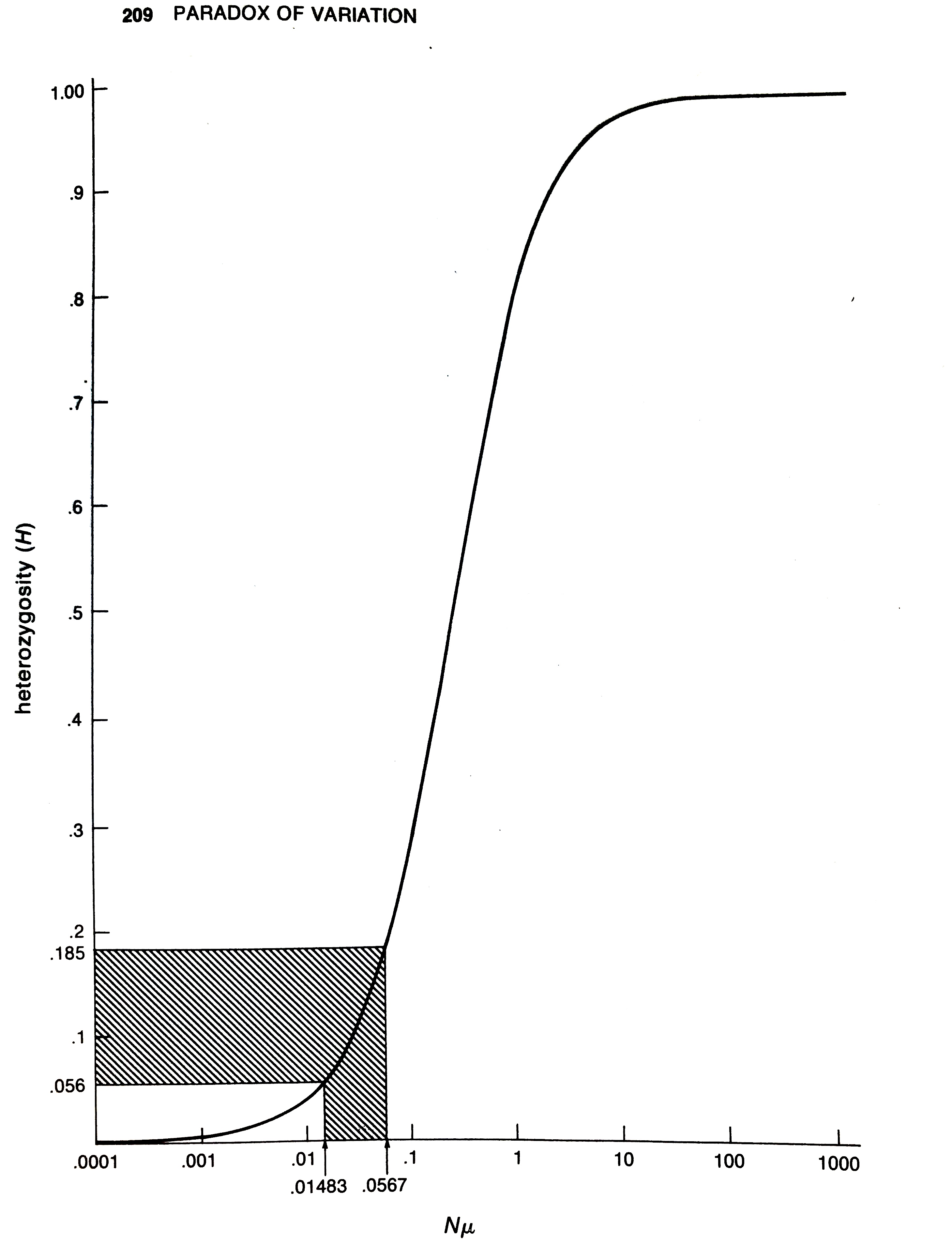
As Lewontin explains,
The observed range of heterozygosities over all the species […] lies in the sensitive region, between 0.056 and 0.184. This range corresponds to values of \(N\mu\) between 0.015 and 0.057. Since there is no reason to suppose that mutation rate has been specially adjusted in evolution to be the reciprocal of population size for higher organisms, we are required to believe that higher organisms including man, mouse, and Drosophila and the horseshoe crab all have population sizes within a factor of 4 of each other. […] The patent absurdity of such a proposition is strong evidence against a neutralist explanation of observed heterozygosity.
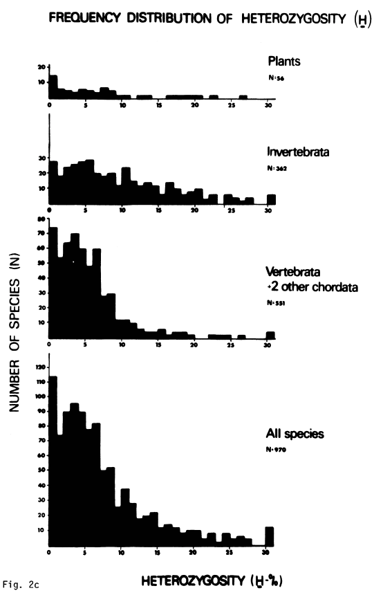
While Lewontin’s estimated range of heterozygosities only included 13 species (Table 22, p. 117), this problem wasn’t just an artifact of small sample size. Throughout the 1970s, estimating protein heterozygosities with gel electrophoresis became a cottage industry. In the decade since Lewontin’s book, over a thousand species had published estimates of their protein variability, which confirmed the narrow range of genetic variability found by Lewontin. Nevo and colleagues published a survey of estimates of protein heterozygosities for 1,111 different species, finding that heterozygosity ranges only from 0% to 30%:5
So Lewontin’s Paradox of Variation seemed to be a rather serious problem for Kimura’s neutral theory, and soon folks were looking for other evolutionary processes that were consistent with the observed data.
Lewontin’s Paradox and the Hitchhiking Model
Lewontin wrote his book while on sabbatical in John Maynard Smith’s lab at the University of Sussex. The neutral theory was under attack from multiple angles, but especially so in Britain, where a cultural that treasured naturalism and adaptive storytelling fostered the conviction that every genetic variant must have some adaptive benefit.6 As Maynard Smith described,
The whole tradition of British population biology had been, if you find a genetic variability, it must have some kind of selective explanation, and if at first you don’t find it, you must try, try, and try again until you do.
Perhaps in the spirit of this tradition, Maynard Smith and John Haigh tried to find a selective explanation for the observed narrow range of diversity diversity. In 1974, they published their masterwork The hitch-hiking effect of a favourable gene, which develops a mathematical model of how a selected variant can decrease its surrounding genetic variability. When a new strongly selected mutation occurs, it does so on a random chromosome in the population. As this mutation increases in frequency, either by improving an individual’s odds of survival or number of offspring, it drags along its neighboring stretches of DNA as it spreads within the population. To understand why this is, it may be helpful to think of our DNA as bit like a spool of 8mm film and you can consider our genes as random frames of the motion picture. Most neighboring frames during a scene of the film end up together into the final production, much like if I pass on a genetic variant I inherited from my father, there’s a good chance that variant’s neighbor would also end up in my child. However, occasionally the film editor comes along and cuts the scene short and splices in another scene. So too can a cell’s recombination machinery cut the stretch of my father’s chromosome I’m passing on and splice in my mother’s; suddenly her genetic variants and their neighbors go on to the next generation. Our genomes, after all, are exactly half of each our parents’ genomes, but a random mosaic of our four grandparents’ genomes.

This is recombination, and it’s a vitally important part of the evolutionary process. In particular, how often recombination occurs —how often the scenes of a film are cut and spliced to different scenes— varies across organisms and along the chromosome itself. In regions of high recombination, beneficial variants are quickly spliced off and away from their neighbors, allowing the surrounding genetic variation to persist in the population undisturbed. By contrast, in low recombination regions, a beneficial variant won’t be spliced away from even its furthest neighbors for quite some time, and vast neighborhoods of genetic diversity are wiped out whenever a beneficial mutation comes along and takes over the population. It is precisely this process that Maynard Smith and Haigh thought could be reducing genetic variability along the genome, and explain the narrow range of genetic diversity seen across species. As they say,
[This investigation] can therefore be regarded as a last ditch attempt to save the neutral mutation theory by showing that there is another process which can account for the uniformity of [heterozygosity] between species.
Nearly fifty years of population genetics has indeed shown that hitchhiking can strongly impact genetic diversity within a species. The textbook example is from work a member of my dissertation committee, Dave Begun, did as a PhD student with Chip Aquadro. They showed that there was a striking correlation between recombination rates and genetic diversity in Drosophila melanogaster, which is precisely what one would expect under pervasive hitchhiking. Genetic diversity is highest in high recombination regions, and lowest in low recombination region across the Drosophila melanogaster genome:
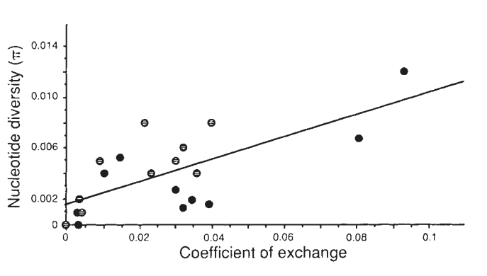
in Drosophila melanogaster, from Begun and Aquadro (1992).
Later, theoretic work showed that a similar reduction in diversity can happen if new mutations are selected against, rather than selected for. This process is called background selection, as it’s continually occurring in the background of the genome. Population geneticists are still debating and developing new ways to estimate the relative strengths of hitchhiking and background selection, which collectively we call linked selection. While hitchhiking and background selection can reduce genetic diversity, and have been shown to do so in many species, the central question remained unanswered: are these selection processes strong enough to constrain genetic diversity across species to the narrow range observed? Or is there some other explanation?
The Neutralist View on Lewontin’s Paradox
Kimura and others had a simpler explanation for the narrow range of diversity. First, we have known since Sewall Wright that what is relevant to the rate of genetic drift, and thus the level of genetic variability, isn’t a species population census size (i.e. the total number of individuals in the population), but rather its effective population size. Effective population size is a bit of an amorphous concept in population genetics, but it’s fundamentally a way to account for the complexities of real populations of breeding individuals. For many populations, the idealized random mating we assume in our mathematical models is overly simplistic and ignores the realities of ecology and demography. Fortunately, we have found that in the vast majority of cases, we can account for the complexities of real populations by simply rescaling the population size, \(N\), to a new “effective population size”, \(N_e\).
Think of it this way: imagine 500 male and 500 female crabs on an island. There crabs freely and randomly mate. Still, it being an island, after a few generations, every crab becomes every other crab’s cousin — remember, the rate at which this happens is proportional to \(1/N\). However, now imagine that a ruthless male despot crab comes along and battles the other males, and forbids them from mating. While there are still \(N=1,000\) individuals on this island, within a generation every crab is the despot crab’s kin. The rate at which every crab on the island becomes a cousin is now much faster. Although this situation seems quite different to the free crab love island, it only requires adjusting \(N\); specifically, we use an effective population size \(N_e\). In this case, it works out that the adjusted \(N_e \approx 4\).7
Importantly, effective population also depends on population bottlenecks. If instead of the male despot crab, the island goes 99 generations undisturbed, but then suffers a severe generation-long bottleneck as seagulls descend on the island. If only 2 crab survive, the effective population size is now reduced from \(N=1,000\) to \(N_e = 170\). Since it’s effective population sizes, and not census sizes, that determine levels of genetic variability, one can see how frequent population bottlenecks could explain Lewontin’s Paradox. The evolutionary history of many species also includes range expansions and colonization and extinctions — when a few individuals make it a new patch of habitable land, procreate, but ultimately may die. These dynamics also decrease effective population size and capture the messy reality of many species.
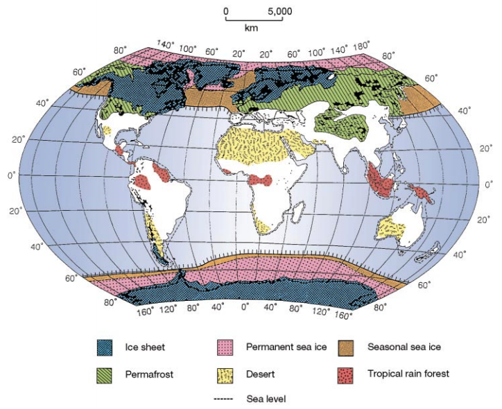
The earth looked very different over the last 20,000 years than it did today. Numerous ice sheets formed and forced species into refugia, where they may have diverged into different species or subspecies (for example, the hooded and carrion crows). This figure is from Hewitt (2000), The genetic legacy of the Quaternary ice ages.
Kimura argued that the only “serious problem that remains to be explained” with Lewontin’s Paradox was that observed heterozygosities never exceeded 30%. Considering Drosophila species, which were at the upper end of the population size and heterozygosity ranges, Kimura argued that their numbers were severely depressed by the last continental glaciation. Genetic variability takes a while to recover from a severe bottleneck, and longer for larger populations (as new mutations must escape rarity and work up to intermediate frequencies), so this severe, lasting bottlenecks during glaciations is the primary neutralist hypothesis for Lewontin’s Paradox.
Recent Work on Lewontin’s Paradox
Technological improvements in genome sequencing revolutionized population genomics, and have provided evidence that diversity within species is shaped by a mix of past demographic events, such as bottlenecks, as well as by natural selection. Lewontin’s Paradox, however, remains unresolved through the genomics era. There are a few nice pieces of recent work that set up some context for my recent paper. The first of which was Ellen Leffler et al. (2012), which compiled estimates of diversity from genomic data. This was one of the first papers I read as I grew interested in population genomics, and certainly inspired me to continue in the field. In this paper, Leffler and colleagues survey diversity for 167 species, and find an 800-fold difference between the highest diversity species (the sea squirt Ciona savignyi) to the lowest diversity species (the wild cat, Lynx lynx). Overall, they point out the narrow range of diversity is still an open and important mystery.
The second paper is J. Romiguier et al. (2014), which surveyed diversity and life-history characteristics across 72 species. These authors find that diversity levels across species are highly-correlated to ecological strategy. In particular they find diversity is highest when species have lots of offspring they invest little in, and lower when species have few offspring they invest more in. Intriguingly, these results suggest ecological processes are predictive of genetic diversity across species. While these ecological correlates are an important piece of the puzzle, it’s still uncertain how mechanistically such ecological processes would act to constrain genetic diversity.
More recently, Russ Corbett-Detig, et al. (2015) tested the hypothesis of whether linked selection could explain Lewontin’s Paradox. Since population sizes are very difficult to estimate for many species, Russ and colleagues considered how the strength of linked selection varies with two proxies of population size: range size and body size. Large-bodied animals (e.g. whales) have smaller population densities than small-bodied animals (e.g. mice), in part because of the energy requirements needed to sustain life are much higher than in larger-bodied animals. Similarly, we’d expect species with larger ranges to have larger population sizes than species with small ranges. Then, the authors fit a statistical model to estimate the strength of linked selection across population genomic samples for 40 species. As a former bioinformatician, I should point out this is a monumental task worthy of praise. Interestingly, they find that the strength of linked selection does seem to scale with these proxies of population size. I read this paper in my first year of graduate school and discussions about it with my PhD advisor Graham Coop were foundational to my early interest in Lewontin’s Paradox.
Graham ultimately found a limitation of Corbett-Detig et al. (2015), which he shared on BioRxiv (Coop 2016). While Corbett-Detig et al. do indeed find that linked selection is stronger in species with large population sizes, it still may not be strong enough to explain why the range of genetic diversity is so narrow. While linked selection was reducing diversity some 60%-80% in species with large population sizes, this isn’t enough to explain why there’s only an 800-fold difference between fruit flies and Lynx, when is likely well upwards of a million-fold difference in their population sizes. The mystery remains open, and at the end of Graham’s article it seemed a bit more likely that repeated bottlenecks and other non-selective processes could also be reducing genetic diversity to the narrow range we observe.
Estimating Census Population Sizes
This brings us to my recent paper in eLife8 that hopefully adds a few more pieces to this longstanding puzzle. My paper tries to chip away at this problem from a few angles, which I’ll detail below. I also tried to include a quick review of the history and relevant literature in my article. Lewontin’s Paradox touches on lots of interesting, and often missed, parts of evolutionary genetics.
The first component of my paper was to try to actually estimate the population sizes across various animal species, and quantify the relationship between genetic diversity and population size. Early work from Soulé (1976), Frankham (1996), and Nei and Graur (1984) has looked at this relationship before, using early protein heterozygosity data:
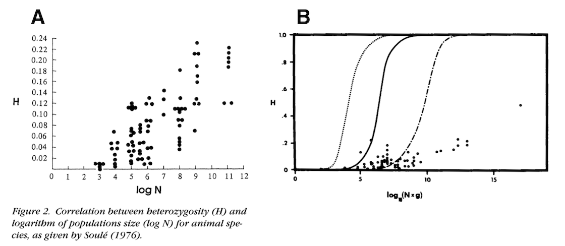
The solid line is neutral expectation if the mutation rate is \(\mu = 10^{-7}\).
These papers used population size estimates from the literature, or back-of-the-envelope calculations. To get a modern look at the relationship between genomic estimates of genetic diversity from previous studies (Leffler et al. 2012, Romiguier et al. 2014, and Corbett-Detig et al. 2015) wanted to find a way to roughly approximate census population sizes for hundreds of species in an automated way. One approach is to take the product of population density (i.e. how many individuals there are per square kilometer) and species range size (i.e. how wide a species range is), to get a very crude estimate of population size. The downside of this approach though, is that population densities are unknown for most species too.
Luckily, the field of macroecology provides a way out. As mentioned, animals have energetic needs that scale with their body sizes. Large-bodied animals require more energy that they procure by hunting or grazing a certain area; competition between individuals for such resources means that large-bodied animals can only live at lower densities. The shocking result is that population densities are surprisingly well correlated with body mass. Damuth (1981, 1987) quantified this; here is a figure from my paper (Figure 1–figure supplement 1):
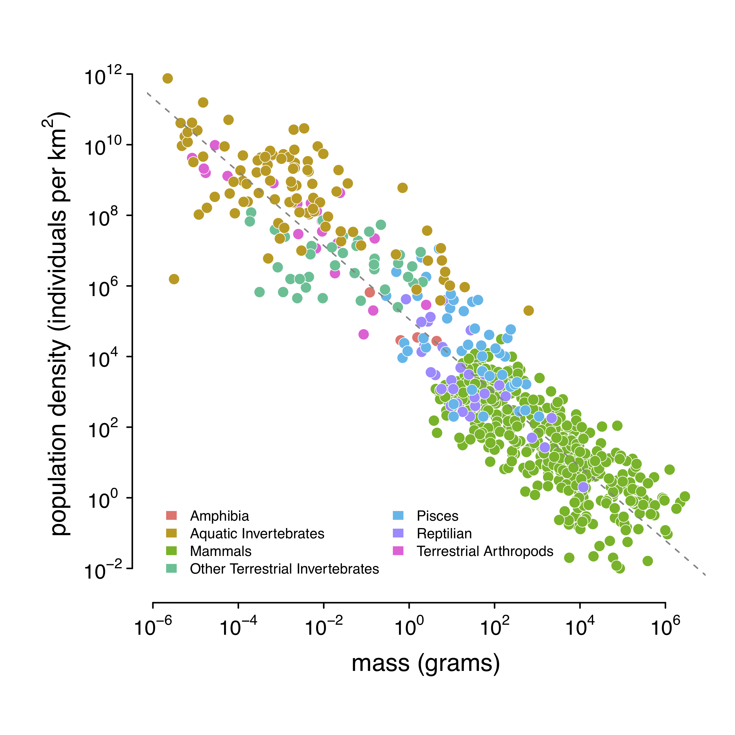
Using this relationship, I predict population density using body mass. In practice, I use body length, since this is much easier to collect and reported in a more standard way than body mass. Using a statistical routine, I predict body mass from body length, and population density from body mass.
Next, I need to estimate range size. A common approach is to use occurrence data —records of the latitude and longitude of where animals were observed— to infer the range. Using the Global Biodiversity Information Facility database, I downloaded occurrence data for the animals species I had genetic diversity and population density estimates for. I then wrote some R code to automatically infer the ranges from this occurrence data.
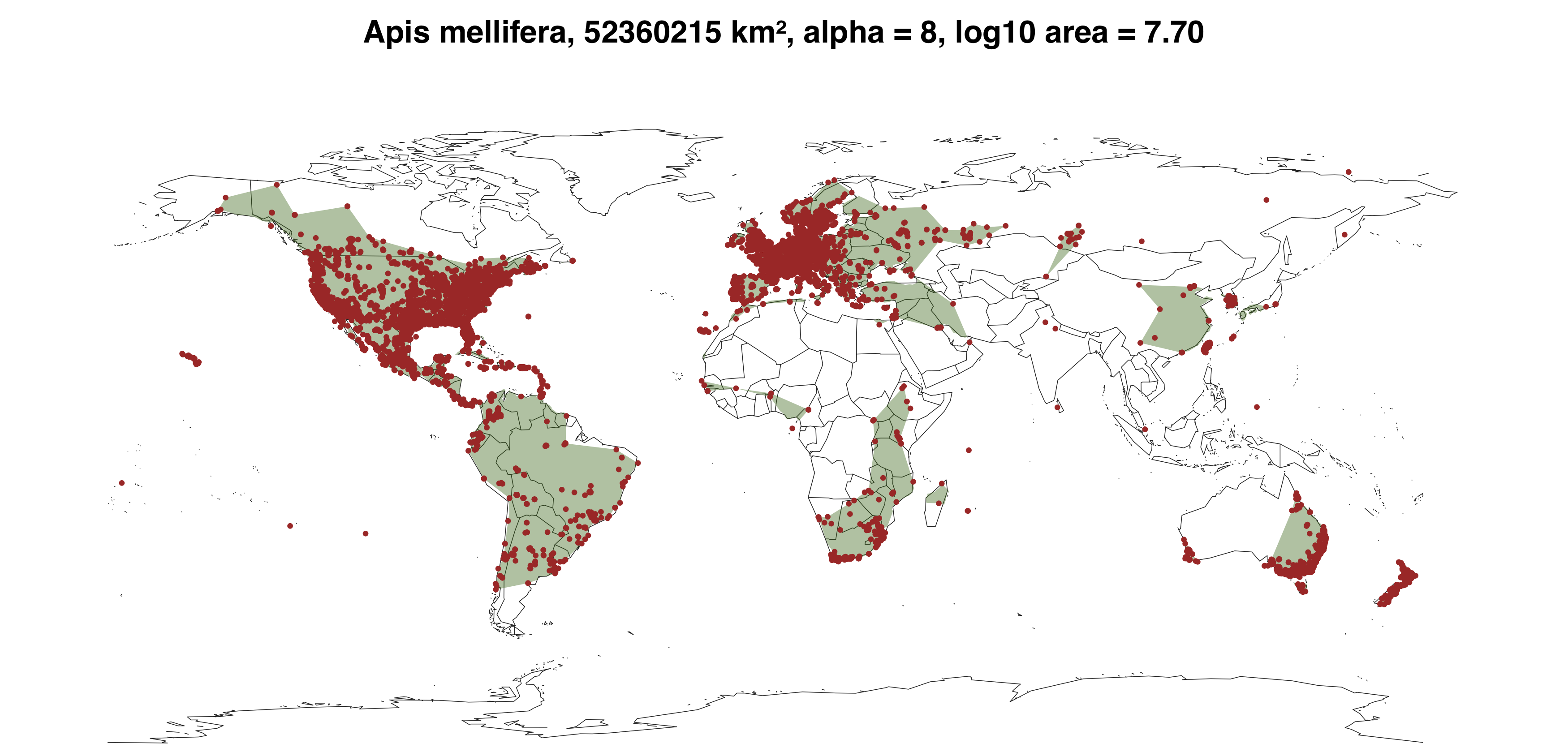
With the population densities and ranges estimated, I take their product to get an approximate population size (see Figure 1 of the paper for a look at the distribution of these ranges by phylum). There’s quite a bit of validation I do to ensure the numerous approximations I’ve made here are reasonable. For example, I make sure my census sizes don’t lead to predictions of the total biomass that are unreasonably small or large (see Population Size Validation and Table 1), since estimates of the total biomass on earth of certain animal groups are available thanks to the study of Bar-On et al. (2018). I also do lots of other consistency checks in Appendix 3.9
The Relationship Between Genetic Diversity and Population Size
Next, I merged the approximate population sizes with the genetic diversity data from Leffler et al. (2012), Romiguier et al. (2014), and Corbett-Detig et al. (2015). These data allow for a nice visualization of Lewontin’s Paradox of Variation, through the relationship between genetic diversity and population size:
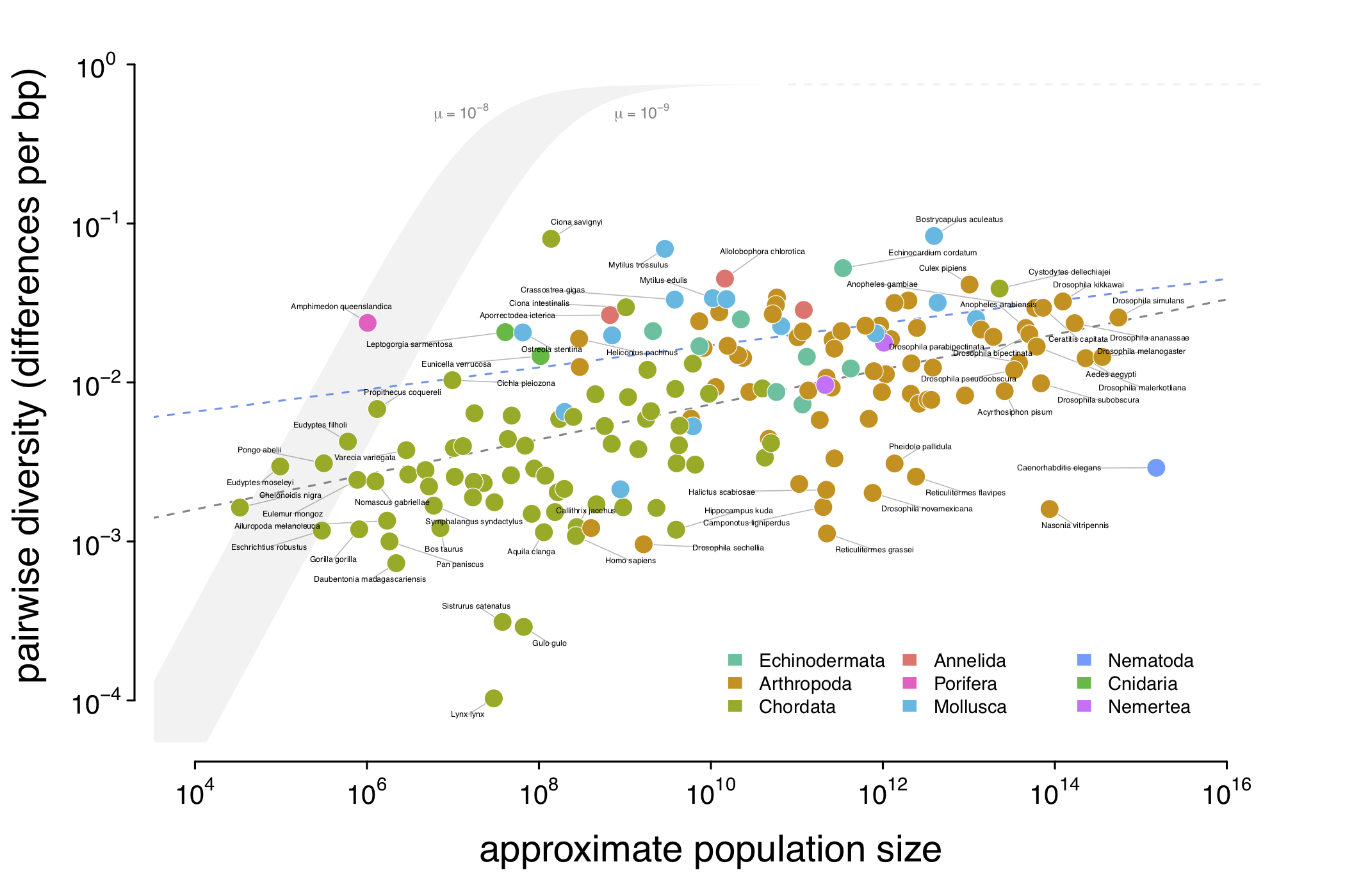
The relationship between genetic diversity (\(\pi\)) and approximate population size (\(N_c\)) for 172 animal species. Note that genetic diversity varies just over three orders of magnitude, while census sizes vary over 12 orders of magnitude. The gray ribbon indicate the expected neutral diversity for a range of mutation rates (\(10^{-9} \lt \mu \lt 10^{-8}\)) were the diversity to be determined entirely by census size under the neutral model. Lewontin’s Paradox wouldn’t be a paradox if the diversity estimates fell in this thin gray area; instead they do not scale with population size, and are mostly constrained to within three orders of magnitude. The eLife article has numerous supplementary figures relevant to this figure here.
What this relationship tells us is that population size appears to impact genetic diversity in the way we’d expected (there is higher genetic diversity in species with larger population sizes – this is shown by the dashed gray line of best fit in the figure above), but as Lewontin first pointed out, genetic diversity doesn’t increase as fast as we’d expect if solely census population sizes and neutral evolution determined genetic diversity.
Is the Diversity–Population-Size relationship meaningful?
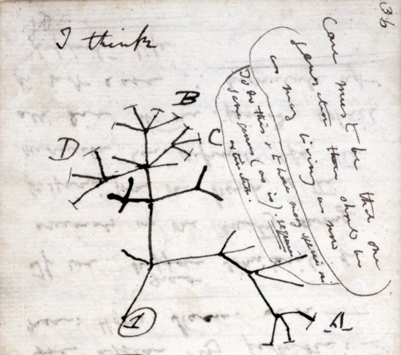
We might look at the relationship above and conclude that there is a significant relationship between population sizes and genetic diversity. Unfortunately, there’s a statistical conundrum that crops up whenever we draw lines of best fit through data points like species. Species are connected by an underlying phylogenetic tree; certain species share common ancestors more recently than others. This was one of Darwin’s brilliant ideas, sketched out in 1837 in his notebook (figure above). In a seminal article in 1985, Joe Felsenstein pointed out that the underlying species tree creates a statistical problem whenever we want to make comparisons across species (as I’m doing here), and this statistical issue should be accounted for.
We can understand this statistical issue, known as phylogenetic non-independence, with a story. Imagine going to a large family reunion, where there are two sides of the family: all the descendents of your great-great-grandfather, and all the descendents of his sister, your great-great-aunt. You look around at all your family members, and observe that there seems to be a statistical relationship between having freckles and being tall. Your tallest relatives tend to have the most freckles, including your great-great aunt’s husband, who towers over you. Other relatives are more average height, and do not have freckles. If you were to collect data and quantify this relationship, you may conclude that somehow these two traits are correlated in a meaningful way; perhaps there’s some biological process that underpins both characteristics.
However, this ignores something: all the relatives that are tall and have freckles descend from your great-great aunt and uncle, and all the average height relatives without freckles descend from your great-great grandfather (who is shorter and doesn’t have freckles). There isn’t necessarily a meaningful relationship between these two traits — it could just be an accident of who shares ancestry (and thus the genes that determine traits) with whom and what traits they happen to have. The family tree here breaks the statistical assumption of independence, since everyone’s related and thus not independent of one another.
This same problem occurs when we compare traits across species too, traits like genetic diversity and census size. John Gillespie, who I introduced at the start of this article, suspected that early pictures of the diversity–population-size relationship may be entirely a spurious artifact of this shared ancestry. In his 1991 book, he has the following figure:

While some previous work has addressed this statistical quandary in clever ways, it’s been limited by the difficulty of building big species phylogenetic trees. In my paper, I use a tool called datelife to build these trees, and then account for this tree structure using something known as Phylogenetic Comparative Methods10. These models account for the way certain groups of related species may all differ from the line of best fit in a systematic way, which is a violation of this statistical model. Overall, I find that even accounting for the species tree, the relationship between population size and diversity is significant statistically. In fact, diversity is also well-predicted by range and body mass (see Supplementary Figure 2–figure supplement 3.
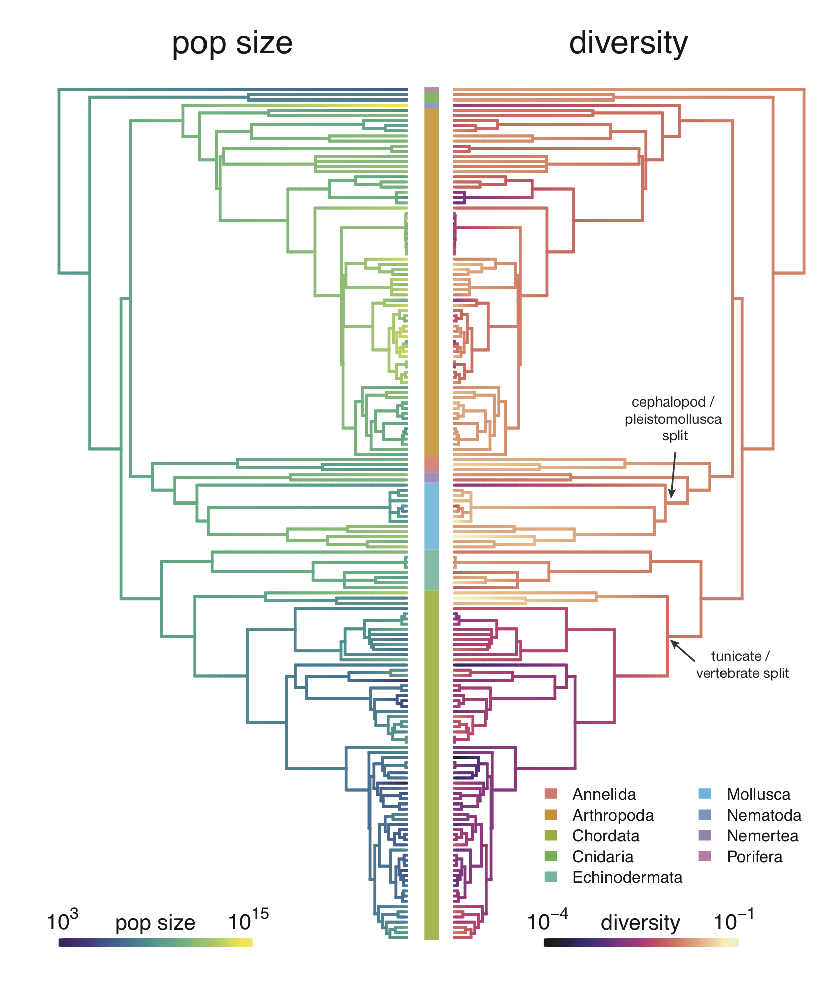
While the relationship between diversity and population size is statistically significant after accounting for shared ancestry, my work finds Gillespie’s concerns are indeed substantiated. Athropods (insects, spiders, and crustaceans) and vertebrates do indeed form to clusters as he suspected. Insects typically have large population sizes and high genetic diversity, while vertebrates typically have smaller population sizes and lower genetic diversity. Still, when I look at the diversity–population-size relationship within each of these groups, I find it is still statistically significant.
There are a few other analyses I did from this macroevolutionary perspective which I won’t discuss here for brevity’s sake. Overall, I came away from this part of the project thinking that considering the Lewontin’s Paradox from a macroevolutionary perspective will be critical in resolving this puzzle. In particular, it may be important to consider how diversity and population size change along the species tree, and how the speciation and extinction processes that lead that give rise to the species we see today interact with genetic diversity and population size.
Can Selection Explain Lewontin’s Paradox?
The final component of my paper is investigating whether selection could explain the shortfall between the observed genetic diversity levels across species, and the diversity we would expect under the neutral theory if effective population sizes were equal to census population sizes (e.g. the gray ribbon in this figure). As described earlier, one of the determinants of how strongly selection can impact genetic diversity is how much recombination there is. The level of recombination varies across species, so if I have any hope roughly predicting how strong selection can get, I need to know how much recombination there is in each species.
Luckily, Jessica Stapley and colleagues published a very nice survey of recombination across animal species. Simply put, the last part of this project wouldn’t have worked without this nice dataset, so I am quite grateful for this work. Using this dataset, I investigated the relationship between recombination map length (the expected number of times chromosomal breaks occur per generation) and my population size estimates. I find that species with large population sizes (such as fruitflies) typically have less recombination (shorter map lengths) than species with smaller population sizes (such as humans). I show this in Figure A below:
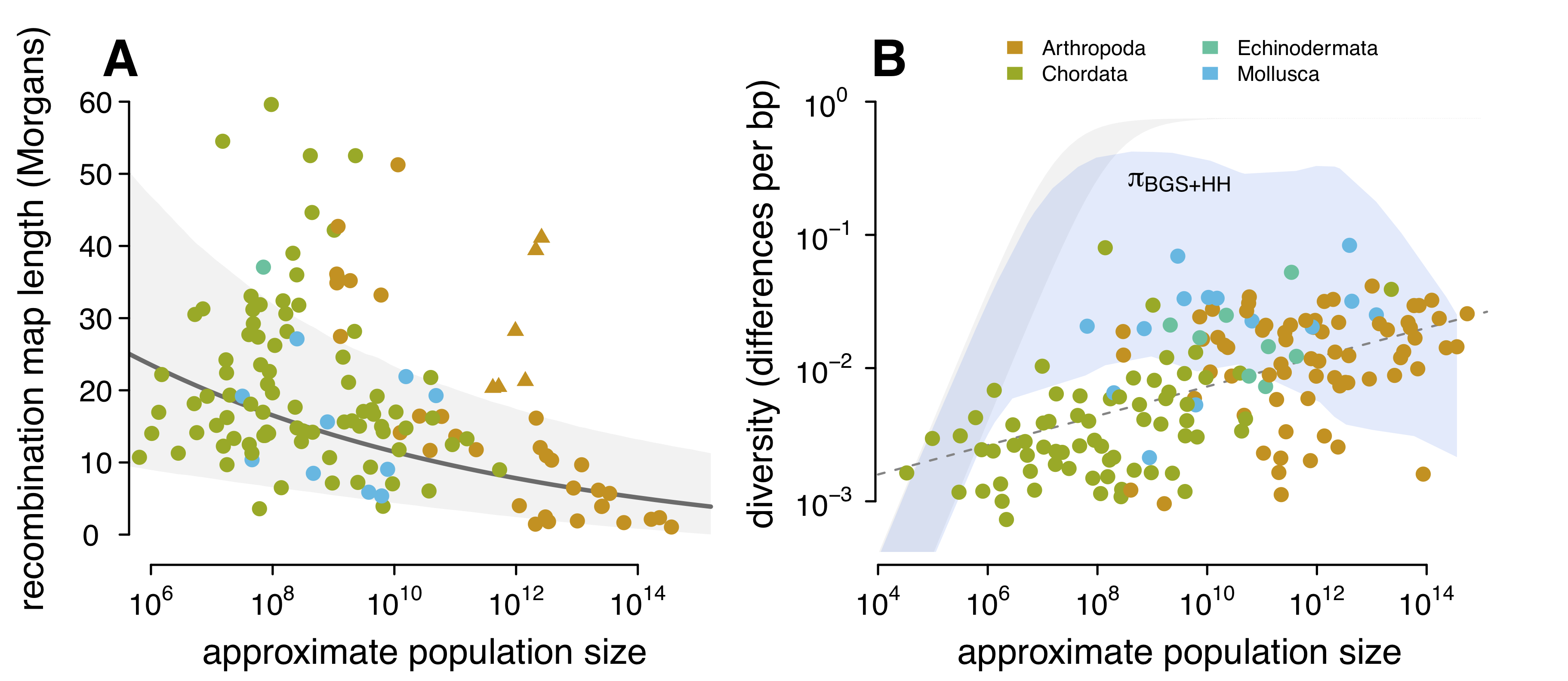
- The relationship between recombination map length and population sizes. These triangle points are eusocial/social species like ants that have adaptively longer map lengths (see Wilfert et al., 2007). (B) The relationship between genetic diversity and population size, with the predicted diversity under hitchhiking and background selection overlaid over it (blue ribbon). The ribbon is the diversity for a variety of mutation rates (\(10^{-9} \lt \mu \lt 10^{-8}\)).
While recombination map lengths are a critical parameter that mediates the strength of selection, there are a few other parameters we unfortunately do not have good estimates of for most species. For example, the rate that new deleterious mutations flow into a population determines diversity, since if more harmful mutations have to be purged from the population, any linked genetic diversity would be purged as well, leading to a net loss of genetic variability. Similarly, we’d also need an estimate of how many beneficial mutations flow into a population each generation, since these also act to reduce diversity through the hitchhiking effect.
While we don’t have estimates of these key parameter for the majority of species in my study, we do have very good estimates for the darling species of evolutionary biology: the fruitfly. In a very nice study by Eyal Elyashiv and colleagues, they developed a sophisticated statistical approach to estimate these key selection parameters for Drosophila melanogaster. Drosophila, with its very large population sizes, has been known to experience some of the strongest selection of any species we’ve looked at. So while I cannot predict the strength of selection for each species, I can predict another useful quantity: if selection were as strong in all species as it is in Drosophila melanogaster, would selection sufficiently reduce diversity to recreate the diversity–population-size relationship I see in the data? It turns out, the answer is no (see Figure (B) above). Essentially, there is too much recombination in species with moderate population sizes — even if we assume they experience absurdly high levels of selection, similar to what we expect in Drosophila, the reduction in genetic diversity caused by selection is severely weakened by the large amount of recombination they experience. It seems that using our current models of linked selection, there is not a plausible way that Lewontin’s Paradox could be solved by selection. In this sense, my work extends Graham’s work: not only do current estimates of the strength of selection seem incapable of explaining the narrow range of diversity, no plausible estimates seem like they could. Indeed, I even try to increase all the key selection parameters ten-fold (Figure 4–figure supplement 3, and still fail to see that predicted diversity matches the observed diversity).
So How Do We Solve Lewontin’s Paradox?
So where does this leave us? From my perspective, my work strengthens the arguments against selection as an explanation for Lewontin’s Paradox. Alternative hypotheses, such as the effect of complex demographic histories like repeated bottlenecks, appear to be a more likely explanation for Lewontin’s Paradox. I also suggest in the discussion that some interaction of macroevolutionary processes, like speciation and extinction dynamics, could play a role in the pattern of diversity we see across species today. At the heart of the problem is that the genetic diversity across species we see today is the result of multiple overlaid processes occurring at very different timescales: ecological, evolutionary, and historical. As I argue in the conclusion, Lewontin’s Paradox may not be fully resolved for some time because the explanation requires synthesis and model building at so many different disciplines.
—and inseparability— of genotype and environment. Source: Why Evolution is True.
Finally, I should mention that while this paper was in its second round of reviews, Dick Lewontin passed away. I was deeply saddened by this news, as were countless of his colleagues, students, and a large number of other younger scientists that were deeply inspired by his work and approach to science. Lewontin was not just a preeminent scientist, but an activist and outspoken opponent of the misuse of genetics for racist ends. He practiced science in a way that was always keenly aware of its larger social context. This is now much more commonplace than it used to be, in part thanks to him. I suggest reading his takedown of Arthur Jensen’s racist misuse of genetics, The Apportionment of Human Diversity, and the The Analysis of Variance and The Analysis of Causes. I’ll never forget reading Lewontin and Cohen (1969) when I took Sebastian Schreiber’s population ecology course during graduate school, nor Lewontin’s chapter in the textbook Building a Science of Population Biology (which I reference at the end of my article). The obituaries in the New York Times, Nature, and the Society for Molecular Biology and Evolution are well-worth reading. Jerry Coyne’s stories of the lab cultural and life of Lewontin are particularly fun to read.11