Using Bioconductor to Analyze your 23andme Data
Bioconductor is one of the open source projects of which I am most fond. The documentation is excellent, the community wonderful, the development fast-paced, and the software very well written.
There’s a new package in the development branch (due to be released as 2.10 very soon) called gwascat. gwascat is a package that serves as an interface to the NHGRI’s database of genome-wide association studies.
Loading the package with library(gwascat) creates a GRanges instance of SNPs and their diseases. GRanges is a fundamental data structure in Bioconductor (specifically the GenomicRanges package) that is designed to hold ranges on genomes efficiently, as well as metadata about the ranges. In this case, the object gwrngs holds SNP ranges (well, locations) and metadata provided by the GWA studies in NHGRI’s database.
While I really do like 23andme’s interface to one’s genotype information and research, the gwascat package offers some nice data mining power. I’ll briefly introduce it here, and perhaps add additional details later on.
23andme Raw Data
When I was considering 23andme, I ultimately persuaded by the fact that they release their raw genotype calls to users. Unfortunately they do so without SNP call confidence data, but in a personal correspondence with a 23andme representative they stated:
Data reproducibility of our genotyping platforms is estimated at about 99.9%. Average call rate is about 99%. When samples do not meet sufficient call rate thresholds, we repeat the analysis, and/or request a new sample. We do not return data to customers that does not meet our quality thresholds.
The 99.9% figure sounds like a lot, but considering there are 960,545 SNPs being called, it’s not that high.
To retrieve raw data, simply click the “Account” link at the top of the page (after you’ve signed in) and click “Browse Raw Data”. There should be a download link. If you’ve never used GPG to encrypt a file, now is the time to learn; keep your SNP data encrypted.
The file 23andme provides has four columns: rs ID, chromosome, position, and genotype.
Loading Raw Data into R
Use read.table to load this data in R. It’s a lot of data, so providing this function with information about the type of data can speed this up quite a bit. Here is the code I used:
library(gwascat)
d <- read.table("data/genome_Vince_Buffalo_Full_20120313162059.txt",
               sep="\t", header=FALSE,
               colClasses=c("character", "character", "numeric", "character"),
               col.names=c("rsid", "chrom", "position", "genotype"))
You may notice that chromosome has the class “character” - this is because there are chromosomes X, Y, and MT (for mitochondrial). For later plotting purposes, it’s good to make this an ordered factor:
tmp <- d$chrom
d$chrom = ordered(d$chrom, levels=c(seq(1, 22), "X", "Y", "MT"))
## It's never a bad idea to check your work
stopifnot(all(as.character(tmp) == as.character(d$chrom)))
Where are the SNPs 23andme Genotypes?
Using Hadley Wickham’s excellent ggplot2 package, we can look at the distribution of SNPs by chromosome:
ggplot(d) + geom_bar(aes(chrom))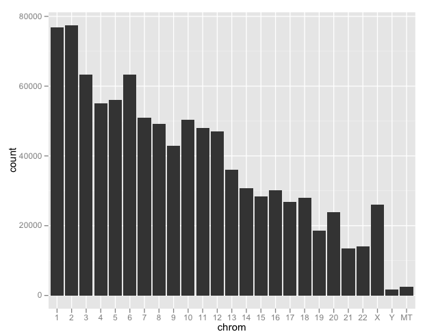
This isn’t providing information on SNP density as much as it is chromosome length (except X). We’ll take a more detailed look a bit later.
Another really wonderful aspect of Bioconductor is that the project isn’t just a repository of code: it also stores annotation, full genomes, and experimental data. Such packaged data is the foundating of reproducible bioinformatics, as you no longer have to worry about keeping track of data versions and storing downloaded data yourself. If you need to work with cutting edge data from Ensembl or UCSC tracks, the packages biomaRt and rtracklayer work well.
A Quick Demonstration of GenomicRanges and Bioconductor Annotation Packages
Suppose I want to see if any of my SNPs fall in the APOE gene region. For this, I’ll need transcript annotation data. If I wished to create a fresh database of exon, gene, transcript, and splicing data, I could with the GenomicFeature package. This package has methods for building transcriptDb objects from the Known Gene track from UCSC, as well as Ensembl databases. However, I’ll just use a pre-packaged version, TxDb.Hsapiens.UCSC.hg18.knownGene. I use hg18 rather than hg19 because this is the build that 23andme’s coordinates reference.
library(TxDb.Hsapiens.UCSC.hg18.knownGene)
txdb <- TxDb.Hsapiens.UCSC.hg18.knownGene
class(txdb) ## do some digging around!
transcriptDb objects have nice accessor functions for accessing their components. Behind the scenes, everything is in SQLite and very efficient (are you seeing why I love Bioconductor?).
If we look at the transcripts with the transcripts accessor function, we see it’s a GenomicRanges object:
> transcripts(txdb)

GRanges with 66803 ranges and 2 elementMetadata values:
          seqnames               ranges strand   |     tx_id     tx_name
             <Rle>            <IRanges>  <Rle>   | <integer> <character>
      [1]     chr1     [  1116,   4121]      +   |         1  uc001aaa.2
      [2]     chr1     [  1116,   4272]      +   |         2  uc009vip.1
      [3]     chr1     [ 19418,  20957]      +   |        26  uc009vjg.1
      [4]     chr1     [ 55425,  59692]      +   |        28  uc009vjh.1
      [5]     chr1     [ 58954,  59871]      +   |        29  uc001aal.1
      [6]     chr1     [310947, 310977]      +   |        33  uc001aaq.1
      [7]     chr1     [311009, 311086]      +   |        34  uc001aar.1
      [8]     chr1     [314323, 314353]      +   |        35  uc001aas.1
      [9]     chr1     [314354, 314385]      +   |        36  uc001aat.1
      ...      ...                  ...    ... ...       ...         ...
  [66795]     chrY [25318610, 25368905]      -   |     33721  uc004fwl.1
  [66796]     chrY [25318610, 25368905]      -   |     33722  uc010nxm.1
  [66797]     chrY [25586438, 25607639]      -   |     33731  uc004fws.1
  [66798]     chrY [25739178, 25740308]      -   |     33732  uc004fwt.1
  [66799]     chrY [25949151, 25949179]      -   |     33733  uc004fwu.1
  [66800]     chrY [26012854, 26012887]      -   |     33734  uc004fww.1
  [66801]     chrY [26015033, 26015066]      -   |     33735  uc004fwx.1
  [66802]     chrY [26015782, 26015809]      -   |     33737  uc004fwy.1
  [66803]     chrY [26016792, 26016820]      -   |     33738  uc004fwz.1
To interact with the wealth of data behind a transcriptDb object, we often group individual ranges into groups, leaving us with a GRangesList.
> tx.by.gene <- transcriptsBy(txdb, "gene")
> tx.by.gene
 GRangesList of length 20121:
 $1
 GRanges with 2 ranges and 2 elementMetadata values:
       seqnames               ranges strand |     tx_id     tx_name
          <Rle>            <IRanges>  <Rle> | <integer> <character>
   [1]    chr19 [63549984, 63556677]      - |     61027  uc002qsd.2
   [2]    chr19 [63551644, 63565932]      - |     61033  uc002qsf.1

 $10
 GRanges with 2 ranges and 2 elementMetadata values:
       seqnames               ranges strand | tx_id    tx_name
   [1]     chr8 [18293035, 18303003]      + | 26503 uc003wyw.1
   [2]     chr8 [18301794, 18302666]      + | 26504 uc010lte.1

 $100
 GRanges with 2 ranges and 2 elementMetadata values:
       seqnames               ranges strand | tx_id    tx_name
   [1]    chr20 [42681577, 42713790]      - | 62142 uc002xmj.1
   [2]    chr20 [42681577, 42713790]      - | 62143 uc010ggt.1

 ...
 <20118 more elements>
Holy GRangeList batman! These are the transcripts grouped by gene. There are other methods for grouping by CDS and exons (cdsBy and exonsBy).
The names of the list elements are Entrez gene IDs. We can look up specific genes with another Bioconductor annotation package, org.Hs.eg.db. There are org.* annotation packages for many organisms. You can forge your own and interact with them with the AnnotationDbi package. I’m using a development version of this package that has a new slick SQL-like interface; it will be widely available with the upcoming 2.10 release.
Suppose I want to convert the Entrez Gene IDs to gene names. The “eg” in org.Hs.eg.db refers to Entrez Gene IDs. Printing the org.Hs.eg.db object gives a nice list of information. Let’s look for the APOE gene’s Entrez Gene ID.
> library(org.Hs.eg.db)
>  cols(org.Hs.eg.db)

    [1] "ENTREZID"     "ACCNUM"       "ALIAS"        "CHR"          "ENZYME"
    [6] "GENENAME"     "MAP"          "OMIM"         "PATH"         "PMID"
   [11] "REFSEQ"       "SYMBOL"       "UNIGENE"      "CHRLOC"       "CHRLOCEND"
   [16] "PFAM"         "PROSITE"      "ENSEMBL"      "ENSEMBLPROT"  "ENSEMBLTRANS"
   [21] "UNIPROT"      "UCSCKG"       "GO"
These are the columns we can query out. Certain keys exist: we can access these using keytypes(). Using it all together, we can extract the Entrez Gene ID:
> select(org.Hs.eg.db, keys="APOE", cols=c("ENTREZID", "SYMBOL", "GENENAME"), keytype="SYMBOL")
    SYMBOL ENTREZID         GENENAME
    23200   APOE      348 apolipoprotein E
Now, we can look for this in our tx.by.gene GRangesList. A word of caution: Entrez Gene IDs are names and thus they need to be quoted when working with GRangesList objects from transcript databases.
> tx.by.gene["348"]
  GRangesList of length 1:
  $348
  GRanges with 1 range and 2 elementMetadata values:
        seqnames               ranges strand |     tx_id     tx_name
           <Rle>            <IRanges>  <Rle> | <integer> <character>
    [1]    chr19 [50100879, 50104490]      + |     59642  uc002pab.1
If I had used tx.by.gene[348] the 348th element of the list would have been returned, not the transcript data for the APOE gene (which has Entrez Gene ID “348”).
Now, do any SNPs fall in this region? Let’s build a GRanges object from my genotyping data, and look for overlaps. Before I do, it’s worth mentioning another gotcha about working with bioinformatics data: chromosome naming schemes. Different databases use all sorts of schemes, and you should always check them. 23andme returns just numbers, X, Y, and MT. Let’s change it to use the same as the Bioconductor annotation.
# CAREFUL: use levels() to check that you're making new factor names
# that correspond to the old ones!
levels(d$chrom) <- paste("chr", c(1:22, "X", "Y", "M"), sep="")
my.snps <- with(d, GRanges(seqnames=chrom,
                   IRanges(start=position, width=1),
                   rsid=rsid, genotype=genotype)) # this goes into metadata
Now, let’s find overlaps using, well, findOverlaps:
apoe.i <- findOverlaps(tx.by.gene["348"], my.snps)apoe.i is an object of class RangesMatching. Note that had we not matched chromosome names, Bioconductor gives us a nice warning that sequence names don’t match. We could look at the slots of apoe.i but output can be seen with matchMatrix:
> hits <- matchMatrix(apoe.i)[, "subject"]
>  hits
     [1] 873650 873651 873652 873653 873654 873655 873656 873657 873658 873659
    [11] 873660 873661 873662 873663 873664 873665 873666 873667 873668 873669
    [21] 873670 873671 873672 873673 873674 873675 873676
So in our subject, we have two hits. Let’s dig them up in our SNP GRanges object:
> my.snps[hits]

  GRanges with 27 ranges and 2 elementMetadata values:
         seqnames               ranges strand   |        rsid    genotype
            <Rle>            <IRanges>  <Rle>   | <character> <character>
     [1]    chr19 [50101007, 50101007]      *   |    rs440446          CG
     [2]    chr19 [50101842, 50101842]      *   |    rs769449          GG
     [3]    chr19 [50102284, 50102284]      *   |    rs769450          AG
     [4]    chr19 [50102751, 50102751]      *   |    rs769451          TT
     [5]    chr19 [50102874, 50102874]      *   |    i5000209          GG
     [6]    chr19 [50102904, 50102904]      *   |    i5000208          GG
     [7]    chr19 [50102940, 50102940]      *   |    i5000201          CC
     [8]    chr19 [50102991, 50102991]      *   |  rs28931576          AA
     [9]    chr19 [50103697, 50103697]      *   |  rs11542040          CC
     ...      ...                  ...    ... ...         ...         ...
    [19]    chr19 [50104077, 50104077]      *   |    i5000212          GG
    [20]    chr19 [50104118, 50104118]      *   |    i5000210          GG
    [21]    chr19 [50104129, 50104129]      *   |    i5000213          CC
    [22]    chr19 [50104154, 50104154]      *   |    i5000207          TT
    [23]    chr19 [50104177, 50104177]      *   |    i5000219          GG
    [24]    chr19 [50104180, 50104180]      *   |    i5000218          GG
    [25]    chr19 [50104198, 50104198]      *   |    i5000206          CC
    [26]    chr19 [50104268, 50104268]      *   |    i5000204          GG
    [27]    chr19 [50104333, 50104333]      *   |  rs28931579          AA
Now, we can verify that these SNPs are in the APOE gene using the UCSC Genome Browser (and actually pull open a browser to this spot from R using rtracklayer, but I’ll save that for another time). Be sure to use hg18/build 36! Note that my genotype information is there.
The ApoE4 allele is rs429358(C) + rs7412(C). The most common allele (ApoE3, or e3/e3) is rs429358(T) + rs7412(C) which is what I have (that’s a relief). There’s a lot of established research that shows homozygous ApoE4 (that is rs429358(C/C) + rs7412(C/C)) leads to substantially higher risk of Alzeheimer’s. According to SNPedia, James Watson requested he not learn his genotype at this locus, and Steven Pinker requested his ApoE data be removed from his PGP10 data.
Looking for Risk Variants using gwascat
We can use the metadata provided by gwascat to further look for interesting variants in our 23andme data. I would recommend interpreting this data with caution, as summarizing these findings in a single element metadata data frame is hard: there’s definitely lost information.
The gwrngs GRanges object has lots of metadata you should scan through with elementMetadata(gwrngs). The Strongest.SNP.Risk.Allele is useful for seeing what you’re at risk for. First, using the rs ID as a key, let’s join our SNP data with the gwrngs metadata:
gwrngs.emd <- as.data.frame(elementMetadata(gwrngs))
dm <- merge(d, gwrngs.emd, by.x="rsid", by.y="SNPs")
We can search for the risk allele in the 23andme genotype data with R and attach a vector of i.have.risk to the dm data frame:
risk.alleles <- gsub("[^\\-]*-([ATCG?])", "\\1", dm$Strongest.SNP.Risk.Allele)
i.have.risk <- mapply(function(risk, mine) {
  risk %in% unlist(strsplit(mine, ""))
}, risk.alleles, dm$genotype)
dm$i.have.risk <- i.have.risk
Now that you have this data frame, you can mine it endlessly. You may want to sort by Risk.Allele.Frequency and whether you have the risk. Because there are quite a few columns in the element metadata, it’s nice to define a quick-summary subset:
> my.risk <- dm[dm$i.have.risk, ]
> rel.cols <- c(colnames(d), "Disease.Trait", "Risk.Allele.Frequency",
                "p.Value", "i.have.risk", "X95..CI..text.")

> head(my.risk[order(my.risk$Risk.Allele.Frequency), rel.cols], 1)
            rsid chrom position genotype Disease.Trait Risk.Allele.Frequency
  2553 rs2315504 chr17 36300407       AC        Height                  0.01
       p.Value i.have.risk   X95..CI..text.
  2553   8e-06        TRUE [NR] cm increase
This is a rare variant, but the most important next question is, rare in who?
> dm[which(dm$rsid == "rs2315504"), "Initial.Sample.Size"]
[1] 8,842 Korean individuals
So this clearly doesn’t mean much to me. We can use grep to find studies that mention “European”:
> head(my.risk[grep("European", my.risk$Initial.Sample.Size), rel.cols], 30)One interesting rs ID that popped up in this list of my data is rs10166942, which is lightly linked to migraines (from which I suffer).
Making Graphics with ggbio
ggbio is a new-ish (Bioconductor 2.9) package that produces really nice graphics. Let’s plot the location of all SNPs that gwascat tells me my allele is the “risk” allele (again, strange word choice as some “Disease.Traits” are height). gwascat uses hg19, and ggbio doesn’t have ideogram cytobanding and chromosome position information for hg18 bundled with it (yet?) so we’ll need to work with that.
> library(ggbio)
> p <- plotOverview(hg19IdeogramCyto, cytoband=FALSE)
Now, let’s take the gwrngs object and subset by my risk alleles. Notice how these assignment function elementMetadata<- is overloaded here:
(elementMetadata(gwrngs)$my.genotype <-
   d$genotype[(match(elementMetadata(gwrngs)$SNPs, d$rsid))])

elementMetadata(gwrngs)$my.risk <- with(elementMetadata(gwrngs),
    mapply(function(risk, mine) {
      risk %in% unlist(strsplit(mine, ""))
    }, gsub("[^\\-]*-([ATCG?])", "\\1", Strongest.SNP.Risk.Allele), my.genotype))
Now to plot these regions:
p + geom_hotregion(gwrngs, aes(color=my.risk))